•Dot product (also called inner product) takes two vectors and gives one number by multiplying matching coordinates and adding them. For example, with V=(3,2) and W=(4,-1), the dot product is 3*4 + 2*(-1) = 10. This single number is not just arithmetic; it measures how much V goes in the direction of W. If V points with W, the number is positive; if against, it’s negative; if perpendicular, it’s near zero.
•Geometrically, the dot product equals the signed length of V’s projection onto the line of W, multiplied by the length of W. A projection means “dropping” V onto the line through W like casting a shadow straight down to that line. The sign tells whether the shadow points the same or opposite way as W. This view turns the dot product into a measurement tool along a chosen direction.
•The dot product is symmetric: V·W = W·V. Algebraically, coordinate-wise products don’t care about order. Geometrically, the length of V’s projection onto W times |W| equals the length of W’s projection onto V times |V|; both equal |V||W|cos(theta). This symmetry helps you switch viewpoints to whichever projection is easier to picture.
•The sign and size of the dot product reveal angle information. When vectors are aligned, the dot product is large and positive; when they’re opposite, large and negative; when they’re at right angles, it’s zero. That’s because only the component along the other vector’s line contributes. This gives a simple test for perpendicularity: V·W = 0 means orthogonal.
•“Inner product” means an operation that takes vectors and returns a scalar (a plain number). It contrasts with the cross product (in 3D) which takes two vectors and returns a new vector. Calling it “dot” product emphasizes the simple coordinate rule. Despite the easy formula, the geometry is the real power.
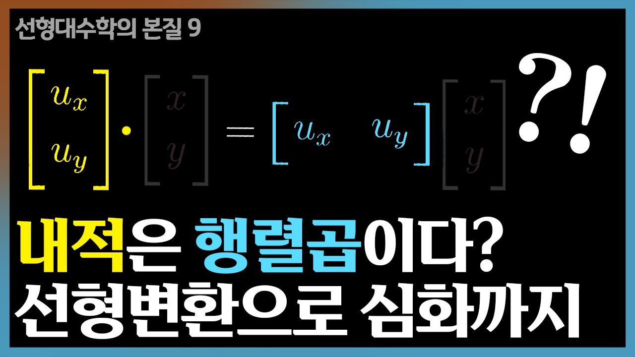
•A linear transformation from n-dimensional space to the 1D number line can be seen as a special kind of measuring machine. Instead of always writing a 1×n matrix (a row vector), you can think of it as: output the dot product with some fixed vector. That fixed vector is the “dual” of the transformation. Each such 1D linear output has a unique associated vector that defines it.
Why This Lecture Matters
Understanding dot products and duality is essential for anyone working with vectors, from students and engineers to data scientists and artists in computer graphics. The dot product gives a fast, reliable way to read alignment, angle, and signed length, which directly powers tasks like testing perpendicularity, projecting forces in physics, calculating work, and computing lighting in 3D scenes. Duality turns any 1D linear scoring rule into a concrete direction-vector, making abstract functions tangible and intuitive. In data and machine learning, this is the basis for linear models: weights form a dual vector that scores inputs by a dot product, linking geometry to prediction. In everyday development, it helps reason about matrix rows as measurement directions and catch mistakes early by visual intuition. Mastering these ideas makes later topics—orthogonal projections, decompositions, and full matrix analysis—far less intimidating. They also enhance career skills by strengthening problem-solving, enabling clear geometric thinking, and improving the ability to explain complex systems simply. As industry leans on linear algebra for graphics, simulation, optimization, and AI, a sharp grasp of dot products and duality is a practical, high-impact advantage.
Lecture Summary
Tap terms for definitions
01Overview
This lesson teaches what the dot product (also called inner product) really is, how to compute it, and—most importantly—what it means geometrically. You begin in a simple 2D setting with concrete vectors V=(3,2) and W=(4,-1), compute their dot product, and then extract the geometry hidden in that single number. The core geometric idea is projection: the dot product equals the signed length of V’s projection onto the line set by W, multiplied by the length of W. This links the size and sign of the dot product directly to how aligned V is with W: aligned gives a big positive value, perpendicular gives something near zero, and opposite gives a big negative value.
A major highlight is symmetry. Algebraically V⋅W = W⋅V because multiplication and addition of matching coordinates work the same in either order. Geometrically, the length of V projected onto W, times |W|, equals the length of W projected onto V, times |V|. Whichever projection is easier to visualize is fine; both give the same number.
The lesson then shifts to why the dot product matters beyond basic calculation: it lets you see 1D linear transformations (maps from Rn to the number line) as dot products with a fixed vector. Instead of thinking of such a transformation as a mysterious function, you can think “measure along this direction.” Any linear transformation that outputs a single number can be written as V ↦ V⋅W for one particular W. This viewpoint is called duality: every such 1D linear map has a corresponding “dual vector” W that fully describes it.
Why does this dual vector always exist? Because dot products are linear in each input: they preserve addition and scaling, just as linear transformations must. This means the behavior of a 1D linear map matches the behavior of taking a dot with some fixed vector. In coordinates, any linear map to 1D looks like y = a1 x1 + a2 x2 + ... + an xn, which is precisely the dot product with a = (a1, a2, ..., an).
Who is this for? The material suits beginners and anyone who wants to finally connect the formula for dot products with an intuitive picture. You only need to know what vectors and coordinates are, plus very basic matrix ideas. No calculus or advanced algebra is required; every concept is anchored to simple geometric drawings and familiar arithmetic.
What will you be able to do afterward? You’ll compute dot products and interpret their sign and magnitude, test for perpendicularity, and find projection lengths. You’ll also recognize that every linear function from Rn to R is just a dot product with some vector, giving you a much clearer mental model of linear transformations. In practical terms, this means you can look at a 1×nmatrix (a row) and instantly picture a direction-vector that “measures” components along that direction.
How is the session structured? It begins with a numeric example to refresh the coordinate rule. Then it builds the geometric meaning via projection and signed lengths. Next it highlights symmetry and discusses the name “inner product” versus other vector products to prevent confusion. Finally, it unfolds the big idea of duality: representing 1D linear transformations as dot products with a specific vector, and motivating why this perspective makes visualization and reasoning easier. The closing notes point ahead to generalizing these ideas to higher-dimensional outputs, where each output coordinate corresponds to its own dual vector (a row of the matrix).
Key Takeaways
✓Always compute and then interpret: get V·W, then ask about sign and size. Predict before calculating: if vectors look perpendicular, expect near zero; if they point together, expect positive. This habit trains geometric intuition and catches arithmetic errors. Interpretation turns numbers into understanding.
✓Use projection formulas to move between numbers and pictures. For pure signed lengths, work with unit vectors: proj_len(V on W)=V·(W/|W|). For the actual projection vector, use ((V·W)/|W|^2)*W. These tools make alignment and decomposition tasks straightforward.
✓Exploit symmetry to simplify visualization. If imagining “V onto W” is awkward, switch to “W onto V”—the final dot product is the same. Choose the viewpoint that makes the geometry clearest. This mental flexibility speeds up reasoning.
✓Normalize when comparing directions across vectors with different lengths. Without normalization, dot products mix in magnitude and can mislead. With unit vectors, the dot product equals cos(theta), a pure alignment score. This is crucial in similarity measures and fair comparisons.
✓Remember that a dot product is always a scalar. If you expect a vector result, you may be thinking of the projection vector or the cross product (3D only). Keep inner vs cross product roles straight. This avoids common mistakes in problem setups.
✓Use the dot product to test orthogonality instantly. Compute V·W; if it’s zero, the vectors are perpendicular. This is faster and less error-prone than trying to measure angles directly. It works in any dimension.
✓Represent 1D linear maps as dot products with a vector. For T(x)=a·x, the row [a1 ... an] and the vector a tell the same story. Draw a as an arrow and think “measure along this direction” to predict signs and magnitudes. This duality makes abstract maps concrete.
Glossary
Dot product (inner product)
A rule that takes two vectors and gives one number. You multiply matching coordinates and add them up. Geometrically, it measures how much one vector goes along the direction of the other. Positive means they point mostly the same way, negative means opposite, and zero means perpendicular. It is the core link between numbers and geometry in vector spaces.
Projection (of a vector onto a line)
Dropping a vector onto a line to see its shadow on that line. The projection shows how much of the vector lies along the line's direction. Its length can be positive or negative depending on direction. The projection vector lies on the line, while the projection length is a signed number. This makes direction and amount easy to read.
Signed length
A length that can be positive or negative to show direction. Positive means the arrow points the same way as a chosen direction; negative means the opposite. It helps keep track of which way the projection points. This is more informative than plain, always-positive lengths. It turns a distance into a direction-aware measure.
Vector length (magnitude, norm)
How long a vector is, computed by the square root of the sum of squares of its coordinates. It’s like the distance from the origin to the point. Bigger length means a longer arrow. Length is always nonnegative. It scales when you scale the vector.
Version: 1
•This idea is called duality: every linear map from vectors to a single number corresponds to exactly one vector under the standard dot product. You feed in any vector V, and the map outputs V·W for a specific W. The map’s behavior is fully captured by W. Thinking this way turns abstract transformations into concrete arrows you can picture.
•Why does this correspondence exist? Because the dot product is linear in each input: (V+U)·W = V·W + U·W and (cV)·W = c(V·W). Linear transformations must preserve addition and scaling in exactly this way. So any map to 1D that is linear behaves like “take a dot with some fixed vector.”
•Visualizing transformations into 1D is often easier through their dual vectors. Instead of imagining the whole action of a row matrix, you draw its associated vector W and think “measure along this direction.” This mental shift simplifies problems and offers geometric intuition. You can quickly predict signs, zeros, and magnitudes based on alignment.
•In coordinates, any linear map to 1D looks like y = a1 x1 + a2 x2 + ... + an xn. That is exactly the dot product with the vector a = (a1, a2, ..., an). So a row matrix [a1 a2 ... an] and the vector a represent the same thing. This ties the matrix view and the geometric view together.
•Example with V=(3,2) and W=(4,-1): V·W = 10. The length of W is |W| = sqrt(4^2 + (-1)^2) = sqrt(17). The signed length of the projection of V onto W’s line is (V·W)/|W| = 10/sqrt(17). Multiply this length by |W| and you get back 10, matching the dot product exactly.
•The symmetry of projection is a powerful mental shortcut. Sometimes it’s easier to picture dropping W onto V’s line rather than V onto W’s line. Either way, the product “projection length × other vector’s length” gives the same dot product. This flexibility lets you pick whichever visualization makes the angle or length comparisons clearer.
•The dot product’s magnitude scales with the lengths of the two vectors and the cosine of the angle between them. That is, V·W = |V||W|cos(theta), tying geometry and algebra together. Using this, you can compute angles or test orthogonality. It also explains why normalizing (making a unit vector) makes dot products equal to pure projection lengths.
•Duality generalizes when mapping to m-dimensional outputs: each output coordinate is itself a dot product with a particular row-vector. In 2D-to-2D, there are two rows, hence two dual vectors, one per output coordinate. Each row is a direction that the transformation “measures” along. Understanding each row vector’s geometry helps you see the whole transformation’s effect.
•Conceptually, a dual vector acts like a ruler laid along its direction. The dot product tells how far along that ruler your vector reaches, with a sign for forward or backward. This measurement perspective is concrete and visual. It turns abstract formulas into lengths and shadows on the plane.
•The name “inner product” reminds us we’re combining vectors to get a number inside the same space, unlike the outer or cross product that give different kinds of outputs. For beginners, the safe takeaway is: inner = number; cross (in 3D) = vector. Knowing which is which avoids confusion. It also helps organize your mental map of vector operations.
02Key Concepts
01
Dot product basics — the arithmetic rule: 🎯 The dot product multiplies matching coordinates of two vectors and adds them up. 🏠 It’s like scoring a test: each answer (coordinate) gets multiplied by a weight, then everything is summed. 🔧 For V=(3,2) and W=(4,-1), compute 34 + 2(-1) = 12 - 2 = 10. 💡 Without this rule, we’d have no simple way to compare directions numerically. 📝 This number becomes the core link to geometry and angle information.
02
Geometric meaning via projection: 🎯 The dot product equals (signed length of V’s shadow on W’s line)×(length of W). 🏠 Imagine shining a light straight onto the line of W and measuring the shadow of V on that line. 🔧 The signed shadow length is (V⋅W)/|W|, positive if it points with W, negative if against. 💡 Without this view, the dot product feels like a random formula; with it, it becomes a measurement tool. 📝 For V=(3,2), W=(4,-1): |W|=sqrt(17), signed projection length is 10/sqrt(17).
03
Sign and angle intuition: 🎯 The sign and size of V⋅W tell how aligned V is with W. 🏠 It’s like checking if two cars drive in the same lane (positive), the opposite lane (negative), or cross at an intersection (zero). 🔧 Large positive means small angle, zero means 90 degrees, large negative means near 180 degrees. 💡 This immediately flags perpendicular directions (V⋅W=0). 📝 Engineers and artists use this to decide if a component should contribute or cancel out.
04
Symmetry of the dot product: 🎯 V⋅W = W⋅V both algebraically and geometrically. 🏠 It’s like measuring with either of two rulers: projecting V onto W or W onto V leads to the same final product with the other ruler’s length. 🔧 Formally, |Vproj_o$$n_W|·|W| = |Wproj_o$$n_V|·|V| = |V||W|cos(theta). 💡 This symmetry lets you pick the easiest projection to imagine. 📝 When one vector is much shorter, projecting the longer onto the shorter may be clearer.
05
Name: inner product vs cross product: 🎯 Inner (dot) product outputs a single number; cross product (in 3D) outputs a vector. 🏠 Think of inner product as a thermometer reading (a number), while cross product is like a wind arrow (a new vector). 🔧 This naming prevents mixing up different kinds of vector combinations. 💡 Confusing them leads to wrong expectations about outputs. 📝 Always check: are you expecting a scalar or a vector?
06
Linear maps to one number (functionals): 🎯 A linear transformation from Rn to R can be seen as “measure along a direction.” 🏠 Like holding a ruler along some arrow and reading how far along it a vector reaches. 🔧 In coordinates, y = a1 x1 + ... + an xn = a⋅x; that row a is the ruler’s direction. 💡 This makes many abstract maps concrete and drawable. 📝 A 1×nmatrix and the vector a tell the same story in two languages (matrix and geometry).
07
Duality — the associated vector: 🎯 Every 1D linear map has a unique vector W so that T(V) = V⋅W. 🏠 It’s like each measuring device secretly being just a ruler pointing somewhere. 🔧 The dot product’s linearity in inputs guarantees such a W exists (under the standard dot product). 💡 This identification turns problems about functions into problems about vectors. 📝 You can replace “mysterious T” with a picture of W and reason visually.
08
Why linearity implies the dot-product form: 🎯 Linearity means T(V+U)=T(V)+T(U) and T(cV)=cT(V). 🏠 Like a fair scale: combine weights first or weigh separately then add—same result. 🔧 The dot product satisfies these exact properties: (V+U)⋅W = V⋅W + U⋅W and (cV)⋅W = c(V⋅W). 💡 So dot products are perfect models for 1D linear outputs. 📝 That’s why you can always rewrite T as a dot with some vector.
09
Projection sign convention: 🎯 The projection length is positive if the shadow points the same way as W, negative if opposite. 🏠 Think of walking along W’s arrow: steps forward are positive, steps backward are negative. 🔧 This makes V⋅W positive with alignment and negative against it. 💡 It encodes direction in a single number. 📝 This is crucial in physics for work and in graphics for lighting calculations.
10
Orthogonality test with dot product: 🎯 Two vectors are perpendicular if and only if their dot product is zero. 🏠 Like two streets crossing at right angles—neither helps you go along the other. 🔧 Zero projection means no component of one lies along the other. 💡 This gives a fast algebraic test for perpendicularity. 📝 You can quickly detect right angles without measuring angles directly.
11
Row matrices as dual vectors: 🎯 A 1×nmatrix acts like a dot product with its coefficient vector. 🏠 The row is your measuring stick; columns are inputs you measure. 🔧 Multiplying [a1 ... an] by x gives a⋅x, a dot product. 💡 Switching between row-matrix and vector views increases flexibility. 📝 It helps when interpreting data weights or features in models.
12
Scaling and length effects: 🎯 Scaling either vector scales the dot product by the same factor. 🏠 Like zooming the ruler or the object—measurements grow in step. 🔧 If W is doubled, |W| doubles, and V⋅W doubles; projection length stays the same only if W is normalized first. 💡 Normalize W (make |W|=1) to read pure projection lengths directly. 📝 Unit vectors turn dot products into clean “how far along?” numbers.
13
Angle formula connection: 🎯 V⋅W = |V||W|cos(theta). 🏠 Like checking how much of V “faces” W using a cosine dial. 🔧 This follows from defining projection length along W and multiplying by |W|. 💡 It converts between vector data and angle data. 📝 You can find the angle theta using arccos((V⋅W)/(|V||W|)).
14
Choosing the easiest projection: 🎯 You can compute the same dot product by imagining either projection. 🏠 If picturing “V onto W” feels hard, switch to “W onto V.” 🔧 Because both equal |V||W|cos(theta), the choice is free. 💡 This trick simplifies problem-solving and drawing. 📝 Especially helpful when one of the vectors is near horizontal or vertical in your sketch.
15
1D visualization advantage: 🎯 Visualizing a number-line output is often simpler than full 2D or 3D transformations. 🏠 It’s like turning a complex scene into a single slider reading. 🔧 The dual vector W lets you imagine this easily: measure along W. 💡 This makes planning and predicting outcomes faster. 📝 Great for sanity-checking signs and magnitudes before computing.
16
Extending to multiple outputs: 🎯 A map to Rm has m rows, hence m dual vectors—one per output coordinate. 🏠 It’s like having m rulers, each measuring along its own direction. 🔧 Each output is a dot product with its row; combined, they form the full matrix-times-vector. 💡 Understanding rows individually builds intuition for the whole map. 📝 This preview sets you up for analyzing higher-dimensional transformations.
17
Why the inner product matters: 🎯 It turns algebra into geometry and back again. 🏠 Like translating between a picture and a sentence. 🔧 With dot products, lengths, angles, and linear maps all connect in one framework. 💡 Without it, vectors are just lists of numbers with no shape. 📝 Mastering this lets you reason quickly and correctly about direction and magnitude.
18
Concrete worked example V=(3,2), W=(4,-1): 🎯 Compute and interpret V⋅W=10. 🏠 Think of laying a ruler along W and asking how far V reaches along it. 🔧 |W|=sqrt(17), projection length of V onto W is 10/sqrt(17); multiply by |W| to get 10. 💡 This confirms the projection picture. 📝 It also shows how sign, length, and angle all live inside one simple number.
03Technical Details
Overall picture and data flow: dot product as a measurement machine
Inputs: two vectors V and W in Rn, represented as coordinate lists V=(v1, v2, ..., vn) and W=(w1, w2, ..., wn).
Geometric output meaning: a single scalar (number) that measures how much V points along W. Equivalently, it is the signed length of V’s projection onto the line through W, multiplied by the length of W.
Data flow: coordinates → arithmetic (products then sum) → scalar → interpret as projection-based measurement.
Choice of viewpoint: either “V onto W” or “W onto V,” both give the same dot product when multiplied by the other vector’s length.
Projection in detail: exact steps and formulas
Define |W| (the length, also called magnitude or norm) as |W| = sqrt(w1^2 + w2^2 + ... + wn2).
Define a unit vector in W’s direction as uW = W/|W| if W=0. A unit vector has length 1.
The signed projection length of V onto W’s line is projlen(V on W) = V⋅uW = V⋅(W/|W|) = (V⋅W)/|W|. This is a pure number telling “how far along W” you go to reach V.
The projection vector of V onto the line through W is projvec(V on W) = projlen(V on W) * uW = ((V⋅W)/|W|^2) * W. This vector lies on the line of W, with direction matching W if the length is positive, opposite if negative.
The dot product relates as V⋅W = projlen(V on W) * |W|. Plugging the formula above: projlen * |W| = ((V⋅W)/|W|) * |W| = V⋅W, confirming consistency.
Angle and symmetry
Define the angle theta between nonzero V and W via cos(theta) = (V⋅W)/(|V||W|). This follows from the projection definition: V⋅W = |V||W|cos(theta).
Signed projection length of V onto W: projlen(V on W) = (V⋅W)/|W| = 10/sqrt(17).
Projection vector: projvec(V on W) = ((V⋅W)/|W|^2) * W = (10/17) * (4,-1) = (40/17, -10/17).
Check: length of projvec times |W| equals dot product: |projvec||W| = (10/√17)√17 = 10.
Linear transformations to 1D and duality
A linear transformation T: Rn → R is a function that satisfies T(V+U)=T(V)+T(U) and T(cV)=cT(V) for all vectors V,U and all scalars c.
In coordinates, any such T can be written as T(x) = a1 x1 + a2 x2 + ... + an xn for some fixed coefficients a1,...,an.
Let a = (a1, a2, ..., an). Then T(x) = a⋅x, a dot product with the fixed vector a. Here, a acts like a “ruler direction,” measuring how much of x lies along its chosen pattern of weights.
The 1×nmatrix form of T is the row [a1 a2 ... an]. Multiplying this row by the column vector x gives the same number as a⋅x. Thus, row matrices to 1D are equivalent to dot products with a specific vector.
Duality viewpoint: associate to each T its dual vector a. Knowing a is enough to predict T’s output on any x by computing a⋅x. Conversely, if you specify a, you have specified T.
Why dot products represent linear maps to 1D (intuitive proof sketch)
Start with T being linear. Evaluate T on basis vectors e1, e2, ..., en, where ei has a 1 in position i and 0 elsewhere.
Let ai = T(ei). Because of linearity, T(x1 e1 + ... + xn en) = x1 T(e1) + ... + xn T(en) = a1 x1 + ... + an xn.
Define a = (a1, a2, ..., an). Then T(x) = a⋅x. No other properties are needed; the form arises directly from linearity and the coordinate system.
This shows existence and uniqueness: the vector a is uniquely determined by what T does to the basis vectors, so each T has exactly one dual vector a in the standard inner product setting.
Practical interpretation and visuals
Picture the dual vector a as a physical arrow in space. To compute T(x), you conceptually measure how much x aligns with a. The more x points in a’s direction, the larger T(x) will be; if x is perpendicular to a, T(x)=0.
Sign: if x points opposite to a, the result is negative. Magnitude: grows with both |x| and |a|; normalizing a to unit length makes T(x) read as pure projection length along a.
Benefit: instead of memorizing a row of numbers, just imagine one arrow and a measurement along it. This turns abstract algebra into concrete geometry.
From 1D to mD outputs (preview)
A linear transformation S: Rn → Rm can be written as an m×nmatrix, whose rows r1, r2, ..., rm each define one output coordinate.
The i-th output is ri⋅x, a dot product with the i-th row vector. Each row is a dual vector describing a 1D measurement along its direction.
Understanding each ri helps you visualize S: for each “ruler” ri, ask how much x aligns with it; putting all m measurements together gives the final output vector.
This approach scales intuition: you don’t have to imagine the full mD change at once, just m separate “projections” measured by the rows.
Clarifying sign conventions and zero cases
If W = 0, the dot product V⋅W is 0 for all V, and projection formulas using W/|W| are undefined (division by zero). In practice, we avoid projecting onto the zero vector because it has no direction.
If either vector is zero, the dot product is zero; there is no alignment information to extract.
If vectors are very small in length, the dot product may be small even if directions align; normalize to unit vectors to compare pure directional alignment.
If you care only about angle, work with unit vectors so V⋅W equals cos(theta) directly.
Common pitfalls and how to avoid them
Mistaking the dot product as giving a vector: remember, it always gives a scalar (a single number). If you need a vector “output” from two vectors, you might be thinking of the cross product (3D only) or a projection vector formula.
Forgetting sign: projection lengths can be negative if the vector points opposite the direction of the ruler vector. Keep track of the arrow direction on W.
Ignoring normalization: if you want pure projection lengths, use unit vectors. If you skip normalization, you will mix in |W| and obscure comparisons across different W.
Confusing rows and columns: for maps to 1D, the row represents the dual vector. Columns are more naturally about how the transformation acts on basis inputs, while rows tell you how outputs “measure” inputs.
Step-by-step guide to compute and interpret a dot product
Step 1: Write vectors V and W in coordinates.
Step 2: Multiply matching coordinates and add to get V⋅W.
Step 3: Compute lengths |V| and |W| if you need geometric interpretation or angles.
Step 4: Get signed projection length of V onto W as (V⋅W)/|W|, or angle using arccos((V⋅W)/(|V||W|)) if both nonzero.
Step 5: If you want the actual projection vector, compute ((V⋅W)/|W|^2)*W.
Step 6: Decide sign and magnitude meaning: positive/negative aligns/anti-aligns; near zero means near perpendicular.
Examples of 1D linear maps as dot products
Consider T(x,y) = 4x - y. Its dual vector is W=(4,-1). For any vector V=(x,y), T(V) = V⋅W = 4x - y.
Consider U(x,y,z) = 2x + 0y - 3z. Its dual vector is A=(2,0,-3). Then U(V) = A⋅V measures a signed combination of x and z components.
If we normalize A to a unit vector, U becomes a scaled measurement of pure directional alignment along A’s direction.
Bringing it together with the main numeric example
V=(3,2), W=(4,-1). Dot product 10 tells us V has a positive component along W’s direction. The projection vector of V onto W is (40/17, -10/17), clearly pointing mostly in W’s direction.
The symmetry means we could instead project W onto V: projlen(W on V) = (V⋅W)/|V| = 10/|V|; multiplying by |V| again returns 10. This switch shows both visualizations encode the same relationship between V and W.
Why this matters beyond the plane
The same reasoning applies in any dimension: dot products always answer “how much along that direction?”
Duality tells you that every linear scoring rule to one number is determined by one vector: a compact, visual, and intuitive package.
In higher-dimensional problems (data science, physics, graphics), dot products detect alignment, make projections, and build full transformations row by row. This foundation supports more advanced concepts like orthogonal projections onto subspaces and decompositions of transformations.
In summary, the dot product is both a simple arithmetic rule and a deep geometric measurement, and duality is the bridge that turns any 1D linear transformation into a concrete direction-vector you can see and reason about. Mastering these ideas lets you compute, visualize, and design linear mappings with confidence.
04Examples
💡
Computing a basic dot product: Input V=(3,2) and W=(4,-1). Multiply coordinate-wise: 34=12 and 2(-1)=-2; add to get 10. Output is the scalar 10. Key point: this matches the projection-based interpretation and sets up further geometric insight.
💡
Projection length from a dot product: Input V=(3,2), W=(4,-1). Compute |W|=sqrt(17) and V⋅W=10, so the signed projection length is 10/sqrt(17). This number tells how far along W’s line V reaches, positive because V has a component in W’s direction. Output: a clear geometric measurement from simple arithmetic.
💡
Projection vector formula in action: Input V=(3,2), W=(4,-1). Compute projvec(V on W) = ((V⋅W)/|W|^2) * W = (10/17)*(4,-1) = (40/17, -10/17). Output is a vector lying exactly on W’s line, pointing mostly the same way as W. Key point: this vector’s length times |W| reproduces the dot product.
💡
Orthogonality test: Input V=(1,2) and W=(2,-1). Compute V⋅W=12 + 2(-1)=0. Output 0 means the vectors are perpendicular. Key point: zero dot product is a fast, exact perpendicularity test.
💡
Angle from a dot product: Input V=(3,2), W=(4,-1). Compute |V|=sqrt(13), |W|=sqrt(17), V⋅W=10, so cos(theta)=10/(sqrt(13)*sqrt(17)). Output theta = arccos(10/sqrt(221)). Key point: dot products encode angle information directly.
💡
Sign meaning: Input V=(−3,−2), W=(4,−1). Compute V⋅W = (−3)4 + (−2)(−1) = −12 + 2 = −10. Output is negative, showing V points mostly opposite to W. Key point: the sign alone tells alignment vs anti-alignment.
💡
Scaling effect: Input scale V by 2 to V'=(6,4) with same W=(4,−1). Compute V'·W = 2*(V⋅W) = 20. Output doubles, confirming linearity in scaling. Key point: scaling either input scales the dot product by that factor.
💡
1D linear map as dot product: Define T(x,y)=4x−y. For input V=(3,2), output T(V)=4*3−2=10, which equals V⋅(4,−1). Key point: the row [4 −1] and vector (4,−1) are the same linear measurement written two ways.
💡
Switching projection viewpoint: With V=(3,2), W=(4,−1), project W onto V instead. projlen(W on V)=(V⋅W)/|V|=10/sqrt(13); then multiply by |V| to get back 10. Output is the same scalar either way. Key point: symmetry lets you choose the easier projection to picture.
💡
Zero vector case: Input V arbitrary, W=(0,0). Compute V⋅W = 0. Output is always zero, but projection formulas onto W break because W has no direction (|W|=0). Key point: never project onto the zero vector; there’s no line to project onto.
💡
Normalization to get pure projection: Input W=(4,−1); unit vector uW=W/|W|=(4/√17,−1/√17). For any V, the pure signed projection length along W is V⋅uW. Output is just a number with the length of W factored out. Key point: normalizing removes scale so you read “how far along?” directly.
💡
Decomposing a 2D-to-2D transformation (preview): Suppose A has rows r1 and r2. For input x, outputs are y1=r1⋅x and y2=r2⋅x. Each output is the measurement of x along a row’s direction. Key point: matrices act as collections of dot-product measurements.
05Conclusion
The dot product is both a straightforward calculation and a powerful geometric measurement. Algebraically, you multiply matching coordinates and add to get a scalar, but geometrically that scalar equals the signed length of a projection multiplied by the other vector’s length. This instantly explains the sign (same vs opposite direction), the test for perpendicularity (zero), and the magnitude’s tie to alignment (via cosines). The symmetry V⋅W=W⋅V appears not just in arithmetic but in the equivalence of projecting either vector onto the other’s line. Together, these facts unify length, angle, and direction into one compact operation.
Viewing linear transformations to one number (Rn→R) through dot products unlocks a key idea: duality. Every such linear map is exactly “take a dot with this fixed vector,” turning abstract functions into concrete arrows you can draw and reason about. This lets you replace a 1×n row with a mental picture: a ruler pointed along a direction, reading how far inputs reach along it. That geometric switch clarifies signs, zeros, and magnitudes on sight, often making problems far simpler to visualize and solve.
To practice, compute dot products for pairs of vectors, sketch their projections, and check your intuition: predict signs and relative sizes before calculating. Try building simple 1D linear maps like T(x,y)=4x−y, drawing their dual vectors, and using them to interpret outputs. Next, generalize to transformations with multiple outputs by analyzing each row as its own “measurement direction,” then assembling the full picture.
For further learning, move on to studying projections onto subspaces, orthonormal bases, and how full matrices can be understood row by row (and later, column by column) using inner products. Explore applications: physics (work, components of forces), computer graphics (lighting and shading), and data science (feature weighting and similarity). The core message to remember is simple and deep: the dot product is a measurement of alignment, and duality turns 1D linear maps into concrete directions. Master these, and many higher-level linear algebra ideas will feel natural, visual, and intuitive.
✓Leverage basis vectors to derive dual vectors. Compute T(ei) to get the coefficients ai, forming a=(a1,...,an). This quickly produces T’s dot-product form. It’s a reliable method for constructing or interpreting linear functionals.
✓Track sign conventions carefully in projections. Positive means same direction as the target vector; negative means opposite. Put an arrow on your target vector in sketches to avoid flipping signs by mistake. Consistent signs prevent downstream errors.
✓Scale awareness: scaling inputs or the measuring vector scales the dot product equally. If you want only directional information, fix one to unit length. This helps design stable comparisons and keeps interpretations clean. It’s especially useful in numerical work.
✓Use angle formulas when angles are needed: theta = arccos((V·W)/(|V||W|)). Check the input range is between −1 and 1 to avoid numerical issues. Use unit vectors to simplify. This is handy in geometry problems and validation checks.
✓Think row-wise for multi-output transformations. Each output coordinate is a dot product with that row’s dual vector. Analyze rows one by one as separate “rulers,” then combine. This modular thinking builds strong intuition.
✓Avoid projecting onto the zero vector. It has no direction, so unit normalization fails. If a vector is extremely small, normalize or rethink the setup. This prevents undefined operations and unstable calculations.
✓Draw to reason: sketch vectors, their projections, and the number line. Mark lengths and signs. Visuals expose mistakes and guide correct algebra. This is a powerful habit even for simple problems.
Unit vector
A vector with length 1. It tells direction only, with no extra size. Dividing a nonzero vector by its length makes a unit vector in the same direction. Unit vectors are useful for pure direction comparisons and projections. They simplify formulas and remove scaling effects.
Orthogonal (perpendicular)
Two vectors are orthogonal if they meet at a right angle. In dot-product terms, their dot product is zero. This means neither has a component along the other. It is a fast test for right angles in any dimension. Orthogonality is a key idea in geometry and algebra.
Angle between vectors
A measure of how much one vector turns to face another. It’s related to the dot product by cos(theta) = (V·W)/(|V||W|). Small angles mean strong alignment; 90 degrees means no alignment; 180 degrees means opposite directions. The angle is always between 0 and 180 degrees. This connects numbers to pictures.
Linearity
A property of a function that respects addition and scaling. If T is linear, then T(V+U)=T(V)+T(U) and T(cV)=cT(V). Linearity makes math predictable and consistent. It matches how dot products behave in each input. Many transformations in science are linear because they combine inputs simply.