🎓How I Study AIHISA
📖Read
📄Papers📰Blogs🎬Courses
💡Learn
🛤️Paths📚Topics💡Concepts🎴Shorts
🎯Practice
📝Daily Log🎯Prompts🧠Review
SearchSettings
Chapter 1: Vectors, what even are they? | Essence of Linear Algebra | How I Study AI
📚 선형대수학의 본질2 / 12
PrevNext
Chapter 1: Vectors, what even are they? | Essence of Linear Algebra
Watch on YouTube

Chapter 1: Vectors, what even are they? | Essence of Linear Algebra

Beginner
3Blue1Brown Korean
AI BasicsYouTube

Key Summary

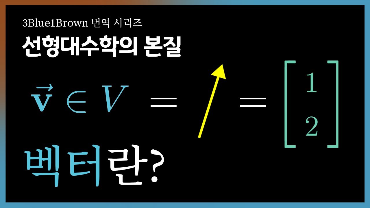
  • •This lesson explains what a vector really is from three connected views: a directed arrow in space, a coordinate like (4, 3), and a list of numbers like [4, 3]. Thinking of vectors as arrows makes direction and length feel natural, while coordinates make calculation easy. Both are the same thing described in different ways. You can move an arrow anywhere without changing the vector, as long as its direction and length stay the same.
  • •A vector in 2D tells you how far to move sideways (x) and up/down (y). In 3D, you also move forward/back (z). The numbers that describe these moves are called coordinates or components, and we often write them as a vertical column. The same vector can have different coordinates if you change the coordinate system (the way you set up your axes).
  • •Linear algebra generalizes vectors to any dimension, even 4D, 100D, or more. You cannot draw higher dimensions easily, but you can still work with them as ordered lists of numbers. Computer science often calls any ordered list a “vector,” which matches this idea. What matters is that the same two operations—vector addition and scalar multiplication—work the same in any dimension.
  • •Vector addition combines movements. Draw the first arrow, then from its head draw the second arrow; the final arrow from the first tail to the last head is the sum. In coordinates, you add each component: (1, 2) + (3, -1) = (4, 1). This head-to-tail rule shows why component-wise addition makes sense.
  • •Scalar multiplication stretches or shrinks a vector. Multiplying by 2 doubles its length; multiplying by 0.5 halves it. Multiplying by a negative number flips its direction while scaling its length. In components, every entry gets multiplied by the same scalar.
  • •Coordinates depend on your choice of coordinate system, like rotating your axes or changing the scale. The vector itself doesn’t change when the coordinate system changes—only its coordinate description does. That’s why it’s sometimes clearer to think with arrows rather than numbers. But numbers are handy for exact calculation.

Why This Lecture Matters

Vectors are the language of direction and change, so learning them clearly helps in many fields. If you work in physics, vectors describe forces, velocities, and accelerations; combining them with addition models net effects. In computer graphics and robotics, vectors describe positions, movements, and orientations; scaling and adding vectors guide animation, camera motion, and robot navigation. In data science and machine learning, each data point is a vector of features; the same component-wise rules let you compute distances and transformations in high dimensions. Even in simple programming tasks, thinking of data as vectors (ordered lists) helps you organize and process information. This lesson solves a common confusion: mixing up a vector with its coordinates or with a point. By separating the geometric idea (direction and length) from its numeric description (coordinates), you avoid mistakes when axes change or when switching between 2D drawings and higher-dimensional lists. The practical skills—head-to-tail addition and scalar multiplication—are the two moves used everywhere in linear algebra, setting you up for span, bases, and linear transformations later. Knowing when to use the arrow picture for intuition and when to use components for exact calculation makes you both fast and accurate. Mastering these basics strengthens your ability to model real problems, communicate solutions, and grow into more advanced topics that power modern technology.

Lecture Summary

Tap terms for definitions

01Overview

This lesson introduces vectors in a way that connects three everyday meanings: arrows in space, coordinates like (4, 3), and lists of numbers like [4, 3]. The goal is to help you see that these are not three different things but three views of the same thing. Each view has strengths. The arrow view makes it easy to feel the direction and length, and it shows how moving the arrow around without changing its direction and length keeps it the same vector. The coordinate view captures the same idea in numbers, which is great for calculation. And the list-of-numbers view lets us work with any number of dimensions, even when we can’t draw them.

This lesson is for beginners who want a solid, intuitive start to linear algebra. No advanced math is needed—only comfort with basic arithmetic and a little geometry. If you’ve plotted points on an x–y graph or moved in a 2D grid, you’re ready. The lesson explains what vectors are, how to add them, and how to scale them (multiply by a number). You’ll also learn that the coordinates we use for a vector depend on how we set up the axes—the coordinate system—but the vector itself is more than just the numbers; it’s the idea of a direction and length (and position change) that those numbers describe.

By the end, you will be able to: recognize and draw vectors as arrows starting from the origin; write vectors as coordinates or as a column of numbers; add vectors using the head-to-tail rule and with component-wise addition; and scale vectors to stretch, shrink, or flip them. You’ll also understand why thinking in both pictures (arrows) and numbers (coordinates) is powerful. With these skills, you’ll be ready for the next key idea: span—how combinations of vectors can reach new places.

The lesson is structured in a natural flow. First, it asks, “What is a vector?” and answers from three viewpoints: an arrow from the origin, a pair/triple/list of numbers, and a general container for ordered data. Then it explains how the same vector can be shifted in space (without changing what it is) and how coordinates track sideways and vertical movement in 2D (and, by idea, depth in 3D). You see that coordinates are a convenient description but depend on the chosen coordinate system. After that, the core operations are introduced. Vector addition is shown with the head-to-tail rule and as “doing two movements at the same time,” which directly matches adding the components. Scalar multiplication is shown as stretching, shrinking, or reversing the arrow and as multiplying every component by the same number. Finally, the lesson emphasizes that these two operations—addition and scaling—are the simple building blocks for all of linear algebra, and it hints at what comes next: span, the set of all vectors you can reach by combining given vectors with these two operations.

Key Takeaways

  • ✓Draw vectors as arrows from the origin to keep their identity clear. If you slide the arrow without turning or stretching, it’s still the same vector. Focus on direction and length; ignore where the arrow is placed. This habit prevents mixing up vectors with specific locations.
  • ✓Write vectors as columns and add them component-wise for quick calculation. Always add top-to-top, bottom-to-bottom (and so on). Check your work with a quick sketch to see if the direction looks right. The geometry and the numbers should agree.
  • ✓Use the head-to-tail rule to add vectors visually. Place the second vector’s tail at the first’s head and draw the resultant from the original tail. This shows addition as doing one movement after another. It’s a reliable way to build intuition before computing components.
  • ✓Scale vectors by multiplying every component by the same number. Positive scalars stretch or shrink while keeping direction, and negative scalars flip direction too. Check extremes: 0 collapses to the zero vector; -1 flips without changing length. Sketching helps lock in the feel.
  • ✓Separate vectors from points in your thinking. A point marks a location; a vector marks a movement. Never add a point to a point thinking it’s vector addition. Use vectors to represent displacements between points.
  • ✓Remember that coordinates depend on your choice of axes. Rotating or rescaling your axes changes the coordinate description but not the vector itself. When something seems to “change,” ask if the axes changed. Keep the arrow picture in mind to stay oriented.
  • ✓Switch between pictures and numbers depending on what’s easiest. Use arrows to reason about direction and combined movement; use coordinates for exact sums and scalings. In higher dimensions, lean on the numeric rules. Let each view support the other.

Glossary

Vector

A vector is a mathematical object that has direction and length. You can picture it as an arrow starting at the origin and pointing somewhere. It shows how to move from one place to another. Vectors are used in any number of dimensions, not just 2D or 3D. They are more about movement and change than about fixed locations.

Arrow representation

This is the picture of a vector as a directed arrow. The tail is at the starting point (usually the origin), and the head shows where you end up. The length shows how big the movement is, and the direction shows where it goes. Sliding the arrow around without turning or stretching it doesn’t change the vector. This makes the drawing focus on direction and length.

Origin

The origin is the zero point in a coordinate system. In 2D it’s (0,0), and in 3D it’s (0,0,0). Vectors are often drawn with tails at the origin because it makes addition and scaling easier to picture. It’s like the home base for directions. Starting from there keeps things simple.

Coordinate

A coordinate is a number that tells you how far to move along an axis. In 2D, you have two coordinates: x (left/right) and y (up/down). In 3D, there are three coordinates: x, y, and z. Together, they describe the components of a vector. Changing axes changes these numbers, but not the vector itself.

#vector#arrow representation#components#coordinates#column vector#head-to-tail#vector addition#scalar multiplication#magnitude#direction#coordinate system#2d vector#3d vector#4d vector#translation#point vs vector#parallelogram rule#negative scalar#displacement#span
Version: 1
  • •A 1D vector is just a number telling you how far and in which direction to move along a line. A 2D vector is an ordered pair, like moving on a flat map left/right and up/down. A 3D vector adds depth, like moving in a room. A 4D vector is still a list of four numbers, even if we cannot picture it.
  • •The two basic operations—addition and scalar multiplication—are the foundation of linear algebra. They define how vectors combine and scale in any space. Everything later, like span, bases, and linear transformations, builds on these two moves. Mastering their geometric and numeric meanings makes later ideas much easier.
  • •When adding vectors, you can also think of doing the two movements at the same time and seeing the total change. This matches component-wise addition: add x’s to x’s and y’s to y’s. The geometry and the numbers always agree. That agreement is the key bridge between pictures and calculations.
  • •You don’t always need coordinates to talk about vectors. Often the arrow picture is enough to reason about results and directions. At other times, a numeric list is simpler, especially in higher dimensions. Understanding both views lets you choose the one that makes the problem easiest.
  • •Negative scaling is a quick way to reverse direction. Doubling then reversing is just multiplying by -2. The size and direction changes are clear in the arrow view and easy to compute in coordinates. Together, these views make vectors feel both intuitive and precise.
  • •This lesson sets up the next topic: span. Once you can add and scale vectors, you can make whole families of vectors. Span will ask, “What set of vectors can we reach by combining given vectors with these two operations?” That idea drives much of linear algebra.
  • 02Key Concepts

    • 01

      🎯 What a vector is: A vector is a quantity with direction and length that you can picture as an arrow starting at the origin. 🏠 It’s like giving directions: “Go 4 steps east and 3 steps north.” 🔧 Technically, a 2D vector is often written as a column [4; 3], where 4 is the x-move and 3 is the y-move. 💡 Without this idea, many problems involving movement and change are hard to describe clearly. 📝 Example: The arrow from (0,0) to (4,3) and the coordinate [4; 3] describe the same vector.

    • 02

      🎯 Arrows can move: A vector is the same even if you slide the arrow somewhere else, as long as the direction and length don’t change. 🏠 It’s like picking up a stick and placing it somewhere else without bending or turning it. 🔧 Formally, vectors are equivalence classes of arrows with the same direction and magnitude. 💡 This lets us focus on how far and which way, not on exact placement. 📝 Example: An arrow from (1,2) to (5,5) is the same vector as one from (0,0) to (4,3).

    • 03

      🎯 Coordinates/components: Coordinates are the numbers that tell you how far to move along each axis. 🏠 Like instructions on a map: move 4 right (x), 3 up (y). 🔧 Written as a column vector, [x; y] records these moves; in 3D it’s [x; y; z]. 💡 Without coordinates, precise calculation is tricky. 📝 Example: A vector moving -2 left and 5 up is [-2; 5].

    • 04

      🎯 Coordinate systems matter: The same vector can have different coordinates if you choose different axes or scales. 🏠 It’s like rotating your map; north and east move with the map. 🔧 Technically, a change of basis changes coordinates but not the geometric vector. 💡 If you forget this, you may think a vector “changed” when only your description changed. 📝 Example: After rotating axes 90°, a rightward vector may look like an upward vector in coordinates.

    • 05

      🎯 Higher dimensions: Vectors can have any number of components: 1D, 2D, 3D, 4D, and beyond. 🏠 It’s like a checklist with more entries; each slot stores one number. 🔧 A 4D vector is [a; b; c; d]; we compute with it the same way, even if we can’t draw it. 💡 This keeps the same rules useful in many fields. 📝 Example: [2; -1; 0; 5] is a valid 4D vector.

    • 06

      🎯 Vector addition (geometry): To add two vectors, place the tail of the second at the head of the first; the arrow from the original tail to the final head is the sum. 🏠 Like walking one set of directions, then continuing with another. 🔧 This is called the head-to-tail rule and works in any dimension. 💡 It shows why addition combines total movement. 📝 Example: Adding [1; 2] and [3; -1] gives the arrow from (0,0) to (4,1).

    • 07

      🎯 Vector addition (components): Add matching components: (x1, y1) + (x2, y2) = (x1 + x2, y1 + y2). 🏠 It’s like adding east steps to east steps and north steps to north steps. 🔧 This follows directly from the geometry of head-to-tail. 💡 Component-wise addition makes calculation fast and exact. 📝 Example: [1; 2] + [3; -1] = [4; 1].

    • 08

      🎯 Scalar multiplication (geometry): Multiplying a vector by a number stretches or shrinks it; a negative flips its direction. 🏠 Like pulling or pushing a spring longer or shorter, and turning it around if negative. 🔧 If v is a vector and k is a scalar, kv scales the length by |k| and flips it when k < 0. 💡 This models resizing movements without changing their basic direction (unless sign flips). 📝 Example: 2⋅[42·[42⋅[4; 3] = [8; 6]; (-1)⋅[41)·[41)⋅[4; 3] = [-4; -3].

    • 09

      🎯 Scalar multiplication (components): Multiply every component by the same number. 🏠 Like doubling each entry in a shopping list. 🔧 If v = [x; y], then kv = [kx; ky]. 💡 It’s fast and matches the geometric picture perfectly. 📝 Example: 0.5⋅[5·[5⋅[-2; 5] = [-1; 2.5].

    • 10

      🎯 1D vectors: A 1D vector is movement along a line; a sign tells the direction. 🏠 Like a thermometer rising (positive) or falling (negative). 🔧 It’s just a single number, but it obeys the same addition and scaling rules. 💡 This shows the vector idea works even in the simplest space. 📝 Example: On a number line, 3 + (-5) = -2 is vector addition in 1D.

    • 11

      🎯 3D and beyond: In 3D, you add forward/back movement to sideways and up/down. 🏠 Like walking in a room instead of on a flat floor. 🔧 Vectors become [x; y; z], but the same rules apply. 💡 The method scales to any dimension. 📝 Example: [1; 0; 2] + [3; -1; 1] = [4; -1; 3].

    • 12

      🎯 Arrows vs. coordinates: Sometimes the picture (arrows) is more intuitive; sometimes numbers are simpler. 🏠 Like using a map for a path but a list for exact steps. 🔧 Both describe the same vector, and you can switch between them. 💡 Choosing the right view makes problems much easier. 📝 Example: To see direction, draw arrows; to calculate sums, use components.

    • 13

      🎯 Lists in computer science: In programming, a “vector” can mean an ordered list that holds many types (numbers, strings). 🏠 Like a row of labeled mailboxes holding different items. 🔧 In linear algebra, we usually keep them as numbers, which lets us add and scale. 💡 This shared idea helps connect math with computing. 📝 Example: A CS vector [7, "cat", true] differs from a math vector [7; 2; -1], but both are ordered lists.

    • 14

      🎯 The essence of linear algebra: Vector addition and scalar multiplication are the two basic moves. 🏠 Like LEGO rules: you can connect pieces (add) and resize pieces (scale). 🔧 Nearly all later concepts build from these two. 💡 Mastering them makes future topics, like span, feel natural. 📝 Example: The span of vectors uses only adding and scaling.

    • 15

      🎯 Direction and length: A vector’s identity comes from its direction and magnitude (length), not where it’s drawn. 🏠 Like recognizing a melody no matter which instrument plays it. 🔧 Translating an arrow doesn’t change the vector; rotating or resizing does. 💡 This keeps the focus on movement, not location. 📝 Example: Sliding the same arrow across the page doesn’t change the vector.

    03Technical Details

    1. Conceptual architecture: three connected views of vectors
    • Geometric (arrows): Picture a vector as an arrow starting at the origin and ending at some point. Its two defining features are direction (which way it points) and magnitude (how long it is). If you slide the entire arrow anywhere in space without turning or stretching it (a translation), you do not change the vector. This idea separates what a vector is from where it happens to be drawn. In 2D, the arrow points from (0,0) to (x,y); in 3D, from (0,0,0) to (x,y,z). In any dimension, the origin-anchored arrow is the cleanest geometric picture.

    • Numeric (coordinates/components): The same vector can be described by listing how far it moves along each axis. In 2D, we record this as [x; y], usually as a column vector. The top entry x is the horizontal change; the bottom entry y is the vertical change. In 3D, we list [x; y; z]. In n dimensions, we write [x1; x2; …; xn]. These numbers are the components or coordinates of the vector.

    • Abstract/list (general dimension): Linear algebra generalizes vectors to be ordered n-tuples of numbers, where n can be any positive integer. This abstraction lets the same rules work in 4D, 100D, or a million dimensions. While the geometric picture becomes hard or impossible to draw in high dimensions, the numeric rules (add matching components, scale all components) still apply exactly the same way. In computer science, the term “vector” often refers to an ordered list container. In math, we usually keep the entries numeric so addition and scaling make sense.

    1. Coordinates and the role of the coordinate system
    • Axes and coordinates: Coordinates describe a vector relative to chosen axes (like x and y). If you rotate, stretch, or otherwise change the axes (the coordinate system), the coordinate description of the same geometric vector changes. This is why the vector is more fundamental than its coordinates; the arrow is the thing, and the coordinates are one way to report it.

    • Dependence on coordinate system: Suppose a vector points 4 units right and 3 units up relative to your current axes: [4; 3]. If you rotate your coordinate axes by 90° counterclockwise, the same physical arrow now looks like it points 3 units right and -4 units up in the new coordinates (the exact formula depends on the rotation). The geometric vector didn’t change; your description did.

    • Practical takeaway: Don’t confuse a vector with its coordinates. Numbers change with the map; the underlying direction and length do not. When you need intuition, draw arrows. When you need precision and computation, use coordinates.

    1. Vector operations A) Vector addition
    • Geometric rule (head-to-tail): To add vectors u and v, draw u from the origin, then from u’s head draw v. The arrow from the original tail (the origin) to the final head is u + v. This matches the idea of performing one movement after another. If u moves you 1 right and 2 up, and v moves you 3 right and 1 down, then u + v moves you 4 right and 1 up overall.

    • Component-wise rule: If u = [u1; u2] and v = [v1; v2], then u + v = [u1 + v1; u2 + v2]. In 3D, u + v = [u1 + v1; u2 + v2; u3 + v3]. In nD, add each matching component. This is fast and aligns perfectly with the head-to-tail picture.

    • Visualization tip: Drawing a parallelogram with sides u and v gives the same sum vector along the diagonal from the origin. This is just the head-to-tail rule seen symmetrically. It reinforces that addition combines both directions at once.

    B) Scalar multiplication

    • Geometric rule: To compute k⋅vk¡vk⋅v (k is a scalar, v is a vector), stretch or shrink v’s length by |k| and, if k is negative, flip its direction. For k = 2, double the length; for k = 0.5, halve it; for k = -1, reverse it without changing length.

    • Component-wise rule: If v = [x1; x2; …; xn], then k⋅vk¡vk⋅v = [k⋅x1k¡x1k⋅x1; k⋅x2k¡x2k⋅x2; …; k⋅xnk¡xnk⋅xn]. Every component scales by the same multiplier.

    • Intuition: Scaling preserves the vector’s line of action unless the sign flips direction. The picture and the numbers line up exactly.

    1. Dimensions and examples
    • 1D: A 1D vector is simply a signed number describing movement along a line. Adding is just normal arithmetic; scaling is multiplying by a number. The rules are the same as higher dimensions but simpler to visualize.

    • 2D: A 2D vector [x; y] moves x units horizontally and y units vertically. You can add two 2D vectors by adding x’s to x’s and y’s to y’s. Scaling changes both x and y together.

    • 3D: A 3D vector [x; y; z] adds forward/back to the picture. You still add and scale component-wise, even though drawing accurately becomes more challenging.

    • 4D and higher: You cannot draw these easily, but the math is the same: add component-wise and scale each entry. Treat the vector as an ordered list. Trust the rules, not the drawing.

    1. Column notation and practical writing
    • Column vectors: It’s common to write vectors as vertical columns to emphasize stacking components: [x; y] rather than (x, y). This format is especially helpful later when multiplying by matrices (not needed yet), but it also makes the idea of “add top with top, bottom with bottom” visually clear.

    • Examples: • [4; 3] means 4 right, 3 up. • [-2; 5] means 2 left, 5 up. • [0; -1] means 1 down.

    1. Bridging geometric intuition and numeric calculation
    • Two stories, one object: The arrow story explains why the rules make sense (e.g., head-to-tail equals total movement). The number story lets you compute quickly. Always check that the two views agree; if they don’t, re-examine your setup.

    • When to pick which view: Use arrows to reason about direction, length, and how motions combine. Use coordinates when you want to compute exact sums or scalings or when the dimension is too high to draw.

    1. Step-by-step guides A) Adding two 2D vectors by drawing
    • Step 1: Draw u from the origin to its head.
    • Step 2: From u’s head, draw v.
    • Step 3: Draw the arrow from the original origin to the final head; that’s u + v.
    • Step 4: Optionally check with components: add x’s and y’s.

    B) Adding two 2D vectors by components

    • Step 1: Write u = [u1; u2] and v = [v1; v2].
    • Step 2: Compute u + v = [u1 + v1; u2 + v2].
    • Step 3: If needed, sketch to confirm the direction looks right.

    C) Scaling a 2D vector by drawing

    • Step 1: Draw v from the origin.
    • Step 2: If k > 1, extend the arrow to be |k| times longer in the same direction. If 0 < k < 1, make it shorter. If k < 0, flip the arrow’s direction and scale by |k|.
    • Step 3: Label the new vector k⋅vk¡vk⋅v.

    D) Scaling a 2D vector by components

    • Step 1: Write v = [x; y] and choose scalar k.
    • Step 2: Compute k⋅vk¡vk⋅v = [k⋅xk¡xk⋅x; k⋅yk¡yk⋅y].
    • Step 3: Optionally sketch to confirm length and/or direction change.
    1. Tips and warnings
    • Don’t mix tail placements when drawing sums: Always place the second vector’s tail at the first’s head for head-to-tail addition.
    • Don’t forget coordinate system dependence: If axes change, component values change, even if the vector doesn’t.
    • Keep signs straight: Negative components move left or down (in 2D) and can easily be misread.
    • Distinguish vectors from points: A point marks a location; a vector marks a movement from the origin. In 2D drawings, the point (x, y) is where the arrow [x; y] would end if it starts at the origin.
    • Choose the best view: Use arrows for intuition and coordinates for computation. Switching back and forth strengthens understanding.
    1. Practice suggestions
    • Draw several vectors and add them using the head-to-tail rule, then verify by component-wise addition.
    • Scale vectors by different positive and negative numbers and sketch the results.
    • Change your axes (e.g., rotate your grid mentally) and think about how the coordinate description would change, even though the vector’s direction and length don’t.
    1. Big picture
    • The entire structure of linear algebra rests on these two operations: addition and scalar multiplication. They let you combine and resize directions. With just these, you can define span (the set of all combinations you can reach), and from span you move toward bases, dimension, and linear transformations. For now, focus on mastering the feel and the formula of adding and scaling vectors. Everything else will click more easily after that.

    04Examples

    • 💡

      Arrow shift example: Draw an arrow from (0,0) to (4,3). Now slide that same arrow so its tail starts at (1,2) and its head ends at (5,5). The direction and length are unchanged, so it’s the same vector. Key point: vectors don’t depend on where the arrow is placed, only on direction and length.

    • 💡

      Coordinate example in 2D: A vector that moves left 2 and up 5 is written as [-2; 5]. If you start at the origin and follow this vector, you land at the point (-2, 5). The coordinate form records horizontal and vertical moves. Key point: components are just step counts along axes.

    • 💡

      Head-to-tail addition example: Let u = [1; 2] and v = [3; -1]. Draw u, then from its head draw v. The direct arrow from the origin to the final head is u + v = [4; 1]. Key point: geometric addition matches component-wise addition (1+3, 2+(-1)).

    • 💡

      Simultaneous movement example: Think of u as “1 right, 2 up” and v as “3 right, 1 down.” Doing both movements together results in “4 right, 1 up.” In symbols, [1; 2] + [3; -1] = [4; 1]. Key point: addition combines total effect along each axis independently.

    • 💡

      Scalar stretch example: Let v = [4; 3]. Then 2⋅v2·v2⋅v = [8; 6]. The arrow doubles in length but keeps the same direction. Key point: positive scaling preserves direction and multiplies length by the scalar.

    • 💡

      Scalar flip example: With v = [4; 3], (-1)⋅v1)·v1)⋅v = [-4; -3]. The arrow keeps the same length but points in the exact opposite direction. Key point: negative scaling flips direction.

    • 💡

      Fractional scale example: If v = [-2; 5], then 0.5⋅v5·v5⋅v = [-1; 2.5]. The arrow becomes half as long and still points the same way (left and up). Key point: scalars between 0 and 1 shrink vectors.

    • 💡

      1D vector example: On a number line, let a = 3 and b = -5. Then a + b = -2, which is the sum of the two 1D vectors. Scaling by -2 gives -2⋅a2·a2⋅a = -6. Key point: 1D vectors obey the same rules as higher dimensions.

    • 💡

      3D addition example: If u = [1; 0; 2] and v = [3; -1; 1], then u + v = [4; -1; 3]. Geometrically, you’d add forward/back movement too, but it’s easier to compute by components. The final vector moves 4 right, 1 down, and 3 forward. Key point: component-wise addition generalizes to any dimension.

    • 💡

      Coordinate system change idea: Suppose a vector points 4 right and 3 up in your current axes. If you rotate your axes by 90°, the coordinates describing that same arrow change. The vector’s direction and length in space stay the same, but the numbers are different. Key point: coordinates depend on the chosen axes.

    • 💡

      Column notation example: Write v = [4; 3] as a column to emphasize that 4 and 3 are stacked and added with matching positions. If u = [-1; 5], then u + v = [3; 8]. The column format reinforces “top with top, bottom with bottom.” Key point: notation can make operations visually clear.

    • 💡

      Draw-and-check example: Compute u + v for u = [-3; 2], v = [5; 4] to get [2; 6]. Then draw u and from its head draw v, and verify the diagonal from the origin to the final head lands near (2,6). The picture and numbers agree. Key point: cross-checking builds confidence.

    • 💡

      Negative with shrinking example: Let v = [6; -2]. Compute (-0.5)⋅v5)·v5)⋅v = [-3; 1]. The arrow flips direction and becomes half as long. Key point: sign flips direction; magnitude scales length.

    • 💡

      Point vs. vector example: The point (4,3) marks a location; the vector [4; 3] marks a movement from the origin to that location. If you start at (10,10) and add [4; 3], you arrive at (14,13). Key point: points are places; vectors are displacements.

    05Conclusion

    This lesson built a clear, connected picture of vectors from three viewpoints: as arrows that show direction and length, as coordinates like [x; y; z] that record movement along axes, and as ordered lists that let us work in any number of dimensions. You learned that sliding an arrow around without turning or stretching it does not change the vector, which shifts attention from placement to the essential features: direction and magnitude. You also saw how coordinates are a convenient description that depend on your chosen axes, while the underlying vector stays the same. With that foundation, the two main operations—vector addition and scalar multiplication—become natural: head-to-tail or component-wise for addition, and geometric stretching/shrinking or component-wise scaling for multiplication. The geometric and numeric views always agree, and switching between them helps you think clearly and compute accurately.

    To put this into practice, draw vectors and add them using head-to-tail, then verify by adding components. Scale vectors by various positive and negative numbers, and notice how direction and length change. Try simple 1D and 2D cases first, then compute with 3D and even 4D lists to get used to higher dimensions. As you grow comfortable, imagine changing the coordinate system and see how the coordinates change even when the vector does not—this strengthens your understanding that vectors are more than their numbers.

    Next steps include exploring span—the family of all vectors you can reach by repeatedly adding and scaling a given set of vectors. Span will deepen your sense that addition and scaling are the only moves you need to build rich structures in linear algebra. From there, concepts like basis, dimension, and linear transformations naturally follow. The core message to remember is simple but powerful: a vector’s identity is its direction and length, not where it sits; coordinates are just one description; and addition and scalar multiplication are the building blocks for everything that comes next. Keep both the arrow picture and the component rules in mind, and you’ll have a strong, flexible foundation for all of linear algebra.

  • ✓Practice with small, clear examples before moving to higher dimensions. Add and scale 2D vectors and sketch them. Then compute in 3D and 4D using components. The same rules work everywhere, so confidence in 2D carries over.
  • ✓Use signs carefully when working with components. Negative x means left; negative y means down (in 2D). A negative scalar flips direction. Double-check signs to avoid simple but common mistakes.
  • ✓When stuck, reframe the problem using the other view. If the numbers feel messy, draw a quick sketch. If the drawing is confusing, write coordinates and compute. Switching views often makes the answer obvious.
  • ✓Confirm your sums by both methods when learning. Do head-to-tail and also add components. Matching answers build trust in your understanding. If they don’t match, re-check tails, heads, and signs.
  • ✓Anticipate span as the next big idea. Know that all you need for span is addition and scaling. These two moves create whole families of reachable vectors. Practicing them now will make span intuitive later.
  • Component

    A component is one entry of a vector’s list of numbers. Each component matches one axis in the coordinate system. Adding vectors means adding matching components. Scaling means multiplying every component by the same number. Components let us compute quickly.

    Column vector

    A column vector is a way of writing a vector as a vertical list. It makes it visually clear which components line up when adding. It’s also handy later for matrix multiplication. The top entry is the first component, and so on down. It’s a clean format for multi-step math.

    1D vector

    A 1D vector is movement along a single line. It’s just one number: the distance and direction along that line. Positive means one way; negative means the other. Even though it’s simple, it follows the same rules as higher-dimensional vectors.

    2D vector

    A 2D vector has two components, usually written [x; y]. It describes movement on a flat plane: left/right and up/down. You can draw it easily as an arrow from the origin. It’s the most common example when first learning vectors.

    +28 more (click terms in content)